At a glance
Model2Vec turns any sentence transformer into a static model — a lookup table of token vectors — that needs no neural forward pass at query time.
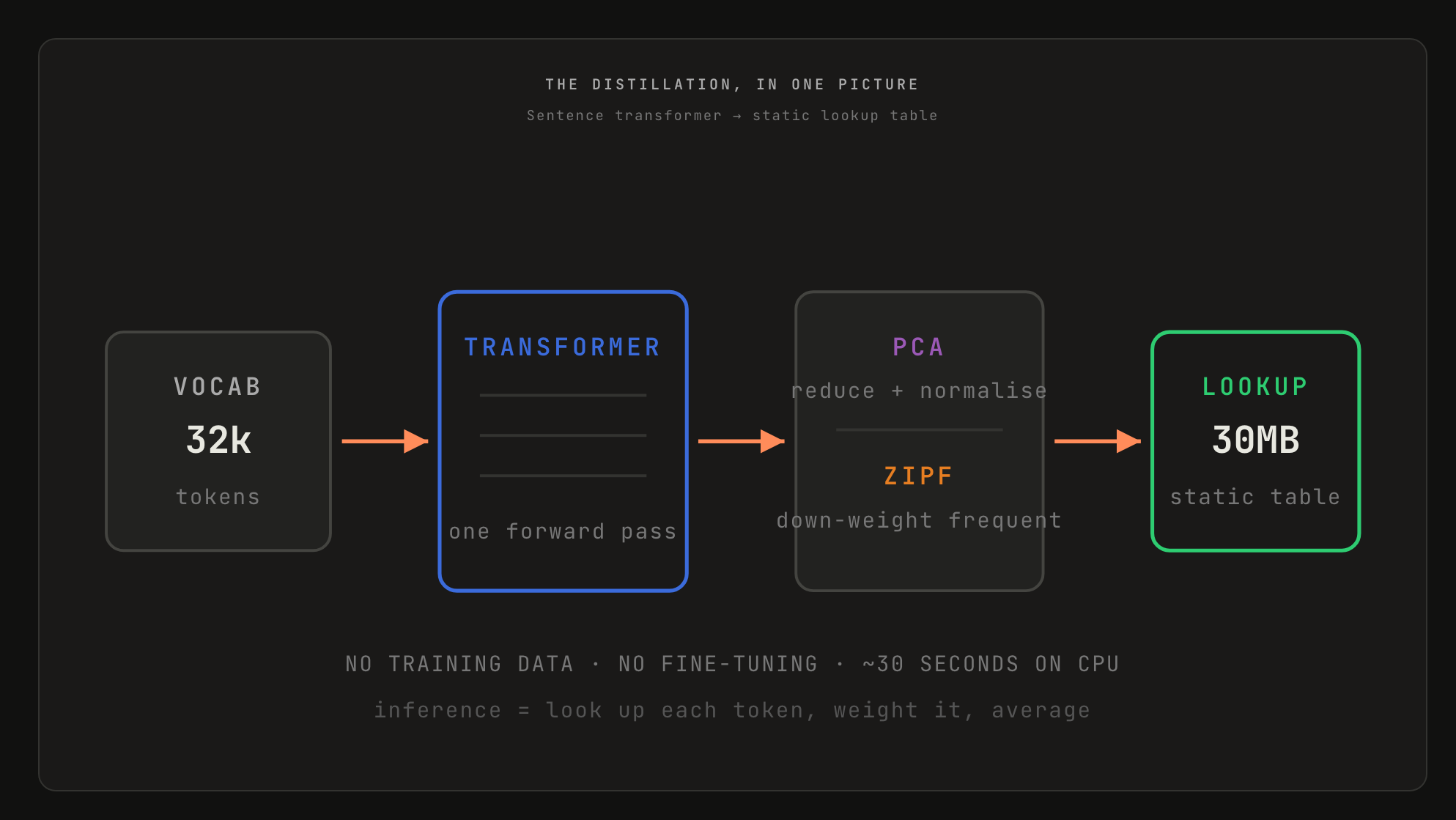
| Metric | Value | Note |
|---|---|---|
| Speed | ~500× faster | vs sentence transformers |
| Size | ~15× smaller | ~30 MB in float32 |
| Time to distill | ~30 seconds | on a CPU, output mode |
| Training data required | None | no dataset, no labels, no gradients |
| Avg score (M2V_base_output) | 46.79 | MTEB + PEARL + WordSim |
| PCA dimensions | 256 | the working default |
The one-line version. The expensive part of an embedding model is recomputing things that never change, and a transformer’s vocabulary is small enough to compute all of them exactly once.
01 Why static embeddings exist
The cost of contextualisation, and who cannot afford to pay it.
Sentence transformers run a full neural forward pass — attention across every token, layer after layer — for every piece of text you encode. That cost is invisible at a hundred documents and is the entire engineering problem at a hundred million, or when a search query must return in under ten milliseconds on a CPU.
The usual escapes are partial. Quantisation shrinks the weights; specialised kernels squeeze the matrix multiplications; distilling into a smaller transformer cuts the layer count. All of them still leave you running a neural network at query time.
Model2Vec takes the other exit: do the neural work once, offline, and never again. Compute the embedding of every token in the vocabulary ahead of time, store the results in a table, and encoding a sentence stops being inference and becomes arithmetic — look up each token, average, done.
The core reframe. A sentence transformer is a function you evaluate at query time. A static model is a table you index into. Model2Vec is the machinery that converts the first into the second — and the surprise is how little you lose in the conversion.
02 How a sentence becomes a vector
Five beats — and the one that Model2Vec swaps out.
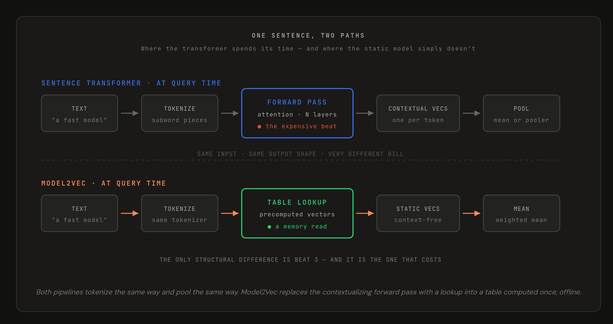
Both pipelines run: text → tokenize → [middle] → vectors → pool. Beats one, two, four and five are effectively identical; the tokenizer is literally the same tokenizer, inherited from the teacher.
What changes is beat three: the transformer contextualises its token embeddings by letting them attend to each other, and Model2Vec does not, because it has already stored one fixed vector per token.
Takeaway. Model2Vec keeps the tokenizer and the pooling and swaps out the middle. The forward pass still happens — once, at distillation time, over the vocabulary — instead of every time you encode a sentence.
03 Two machines, compared
| Sentence Transformer | Model2Vec Static | |
|---|---|---|
| Query cost | Full neural forward pass, every encode | Table lookups plus one average |
| Context | Yes — attention disambiguates each token | None — one fixed vector per token |
| Size | Hundreds of MB | ~30 MB in float32 |
| Hardware | Wants a GPU | CPU is the design target |
| Quality | 56.08 (all-MiniLM-L6-v2) | 46.79 (M2V_base_output) |
Judge it against the right baseline. This is a replacement for GloVe and word2vec, not for your sentence transformer. Against the static baselines it displaces — GloVe at 42.84, BPEmb at 39.34 — it wins on every task measured.
The nine-point gap to MiniLM is the price of the category, not a shortcoming within it.
04 The cache that became a model
How an optimisation turned into an architecture.
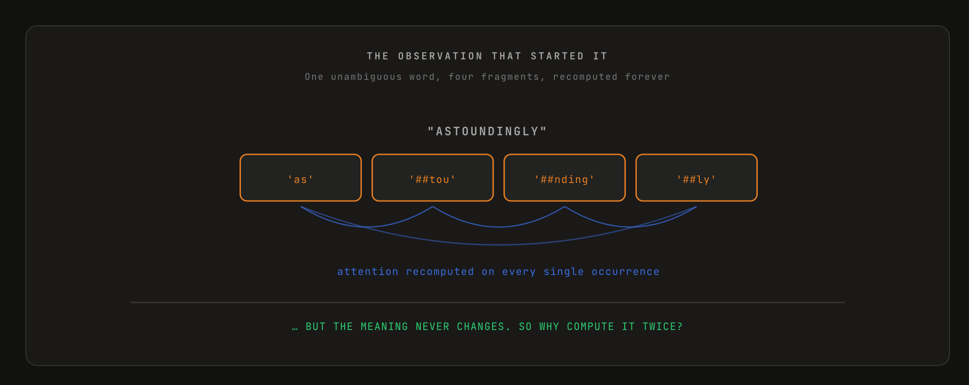
A transformer vocabulary holds only about 32,000 tokens, so longer or rarer words get chopped into pieces. The word astoundingly becomes four subword tokens: 'as', '##tou', '##nding', '##ly'.
Every time it appears, the model recomputes attention among those same four fragments and reassembles the same meaning it assembled last time. That looks like obvious waste, so the original idea was a cache.
Then came the finding that made a caching trick into a method: you do not need to cache whole words at all. The output representations of individual tokens, averaged, already produce good sentence representations.
Run all 32k vocabulary tokens through the model once, store each vector, and throw the model away. The cache became the model.
A 2024 number, re-checked. The ~32k figure is the BERT-family number, and for those encoders it still holds — all-MiniLM-L6-v2 and bge-base-en-v1.5 both carry a 30,522-token vocabulary.
But it is no longer representative. Llama 3 moved to 128k, Gemma to 256k, Qwen3 to ~151k, GPT-4o-era encodings to ~200k. Embedding models inherit those backbones: Qwen3-Embedding ~151k, EmbeddingGemma (Gemma 3) 256k, BGE-M3 (XLM-R) ~250k.
This changes the arithmetic, not the argument. A 256k-token table at 256 dimensions is roughly 250 MB rather than 31 MB, and distillation takes eight times as many forward passes.
Inference speed is unaffected, because cost is per token in your sentence, not per row in the table. A bigger vocabulary also fragments words less, softening the problem in section 11.
05 Distillation — one pass, no data
What actually happens when you run distill().
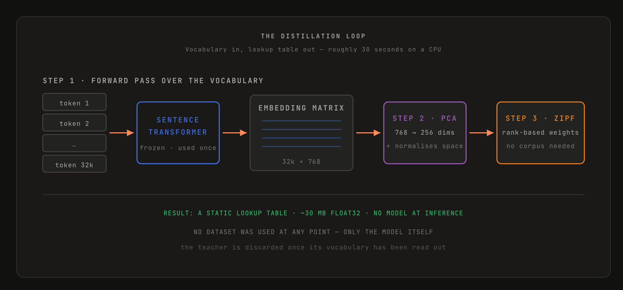
The procedure is three steps. First, pass the vocabulary through the sentence transformer — every token, one forward pass each, collecting the output embeddings. Second, reduce dimensionality with PCA. Third, weight the embeddings using Zipf weighting. That is it.
Zoom in: one entry, start to finish
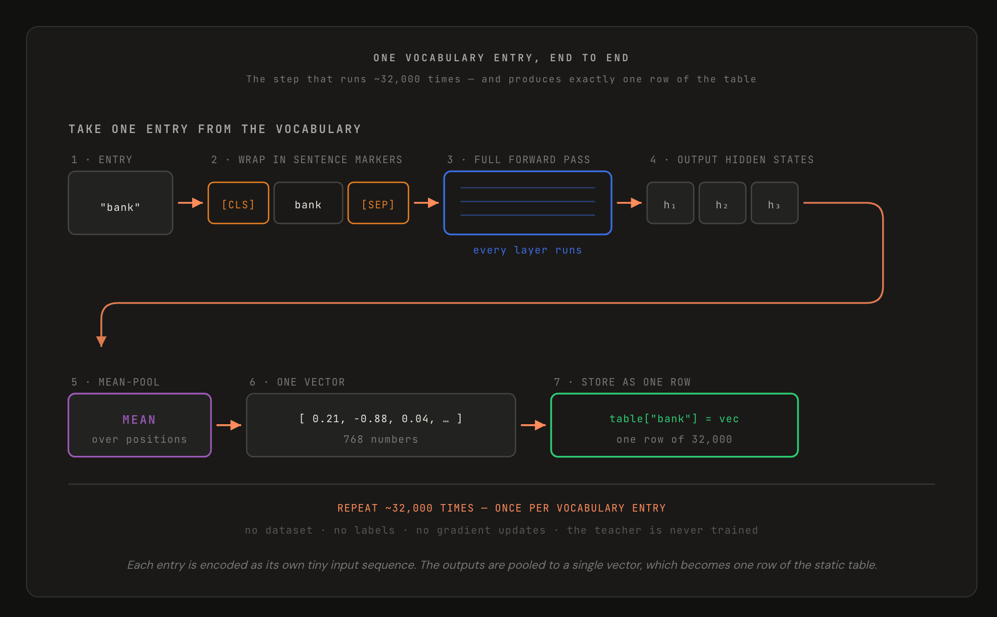
Each vocabulary entry is wrapped in the model’s sentence markers ([CLS] bank [SEP]), pushed through the full network, and its output hidden states are mean-pooled into a single vector, which becomes one row of the table. Repeat ~32,000 times.
There is an objection worth raising, because it makes the method look impossible at first glance. A transformer’s defining trick is letting tokens attend to each other — so if you feed it bank entirely alone, there are no neighbours to attend to. What is the forward pass doing?
Attention is only part of what the network does. Even with nothing to attend to, the token still travels through every layer’s feed-forward blocks, weight matrices and normalisations, and emerges transformed by everything the model learned.
What you store is the model’s context-free reading of the token. The ablations put a number on it: the untouched input embedding scores 40.74, the same token after the forward pass scores 46.79.
What actually goes in. The only required input is the model. The vocabulary comes from its own tokenizer, and the frequency ordering Zipf needs comes from that same tokenizer.
Your data can enter in exactly two optional places, and neither is training: a custom vocabulary (a list of words — no labels, no pairs), and training the finished model afterwards in Sentence Transformers, which is a separate step.
Distillation itself sees neither.
Takeaway. Distillation here means “read out the teacher’s vocabulary and post-process it”, not “train a student”. Because inference no longer runs a network, vocabulary size does not affect speed — a larger vocabulary costs RAM, not latency.
06 PCA — why less is more
Throwing away dimensions that improves the model.
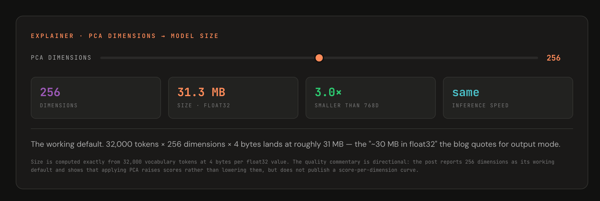
Comparing M2V_base_output_nozipf_nopca at 40.80 against M2V_base_output_nozipf at 43.61, PCA is worth roughly 2.8 points — and it improves results on every task category. You get a smaller model and a better one simultaneously.
The explanation is that PCA does two jobs and only one is compression. The other is normalisation. Transformer embedding spaces are anisotropic — vectors crowd into a narrow cone with a few dominant directions carrying systematic bias rather than semantic content.
PCA re-centres and re-bases the space along its true axes of variation, so cosine similarity starts meaning what you want it to mean.
Dimensionality is also the direct lever on model size, since the model is nothing but a table of vectors: 32,000 tokens × 256 dimensions × 4 bytes ≈ 31 MB.
07 Zipf — weighting without a corpus
Getting IDF’s benefit when you have nothing to count.
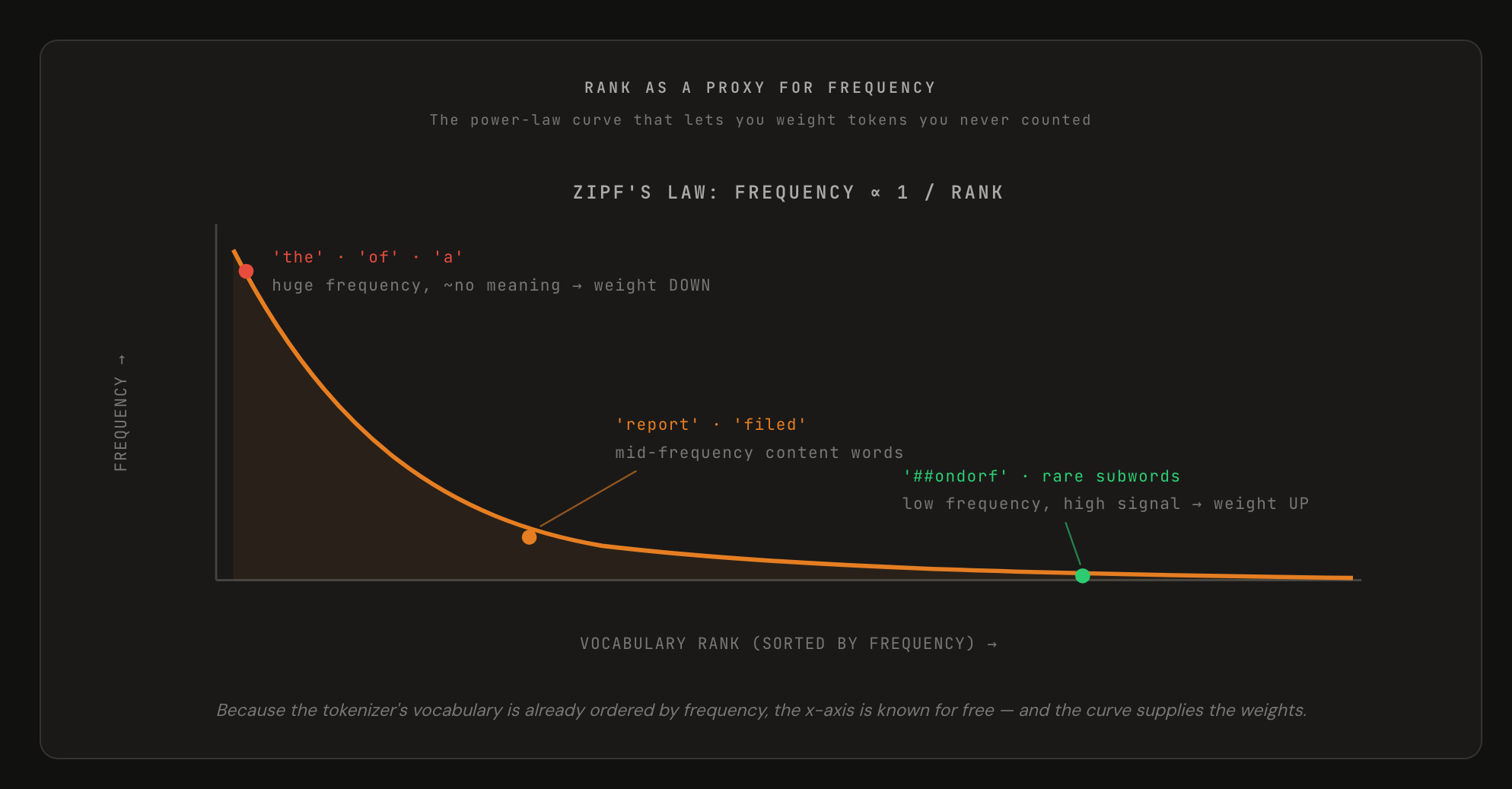
If you average token vectors, weights matter enormously. In “the report on the merger was filed”, words like the, on and was contribute as much as merger and filed — and since function words are also the most frequent, they dominate representations while carrying almost no meaning.
The classical fix is Inverse Document Frequency, but IDF needs a corpus to count in, and Model2Vec’s whole point is that it needs no data. The escape is Zipf’s law: in a frequency-ranked list, frequency follows a power law, so rank alone estimates frequency.
And tokenizer vocabularies are already ordered by frequency — the ranked list is sitting in the tokenizer.
How the weight is actually computed
“Zipf weighting” compresses two ideas. Zipf’s law turns a rank into an estimated probability; a second formula turns that probability into a weight:
# model2vec/distill/inference.py
inv_rank = 1 / np.arange(2, n_embeddings + 2)   # Zipf: frequency is proportional to 1/rank
proba    = inv_rank / np.sum(inv_rank)          # normalise into a probability distribution
weight   = sif_coefficient / (sif_coefficient + proba)   # SIF, default a = 1e-4
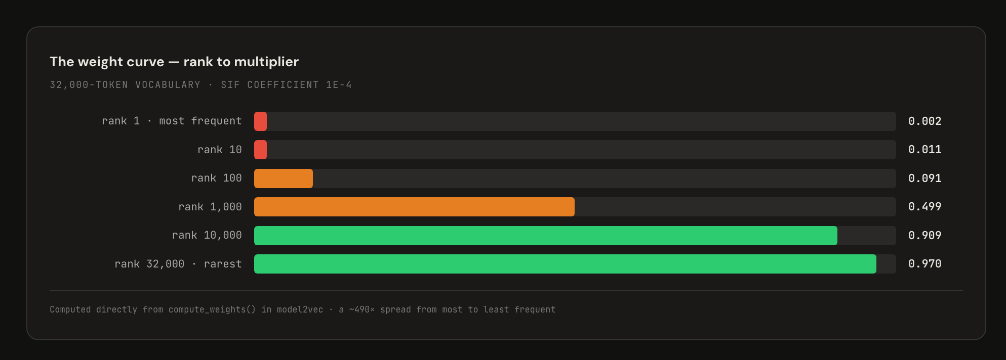
The second line is SIF — Smooth Inverse Frequency (Arora et al., 2017) — the smoothed relative of IDF. As probability approaches zero the weight approaches 1; as probability grows the weight collapses toward 0.
Weights are computed once at distillation and stored beside the vectors, not multiplied into them. Since pooling is a plain mean the arithmetic would be identical either way, so the separation is an engineering choice: Model2Vec can KMeans-cluster the vocabulary so many tokens share one stored vector while each keeps its own weight, and its int8 quantization uses one global scale across the table, which a 490× spread in row magnitude would destroy.
How well are real vocabularies actually sorted? Only the learned wordpieces are frequency-ordered. In bert-base-uncased, ids 0–993 are [PAD] and [unused*] slots (pruned by Model2Vec), ids ~994–1995 are special tokens, punctuation and characters, and **frequency ordering only starts at id 1996 with the, of, **and.
So the lands near rank 1003 and receives a weight of about 0.498 — not the 0.002 the idealised story implies. The tokens crushed at the top of the ranking are mostly punctuation, and function words end up down-weighted only about 2× relative to rare tokens rather than 500×.
It still earns its 3.2 points, but the mechanism is coarser than “IDF without a corpus” suggests. The approximation is better for BPE tokenizers (GPT-2, Llama, Qwen), where merges are learned greedily by frequency.
08 The mean, and what it costs
Living without context — and why it hurts less than you would expect.
At inference there is one operation: look up the vector for each token present, scale it by its frequency weight, and average the results. This makes the model completely uncontextualized.
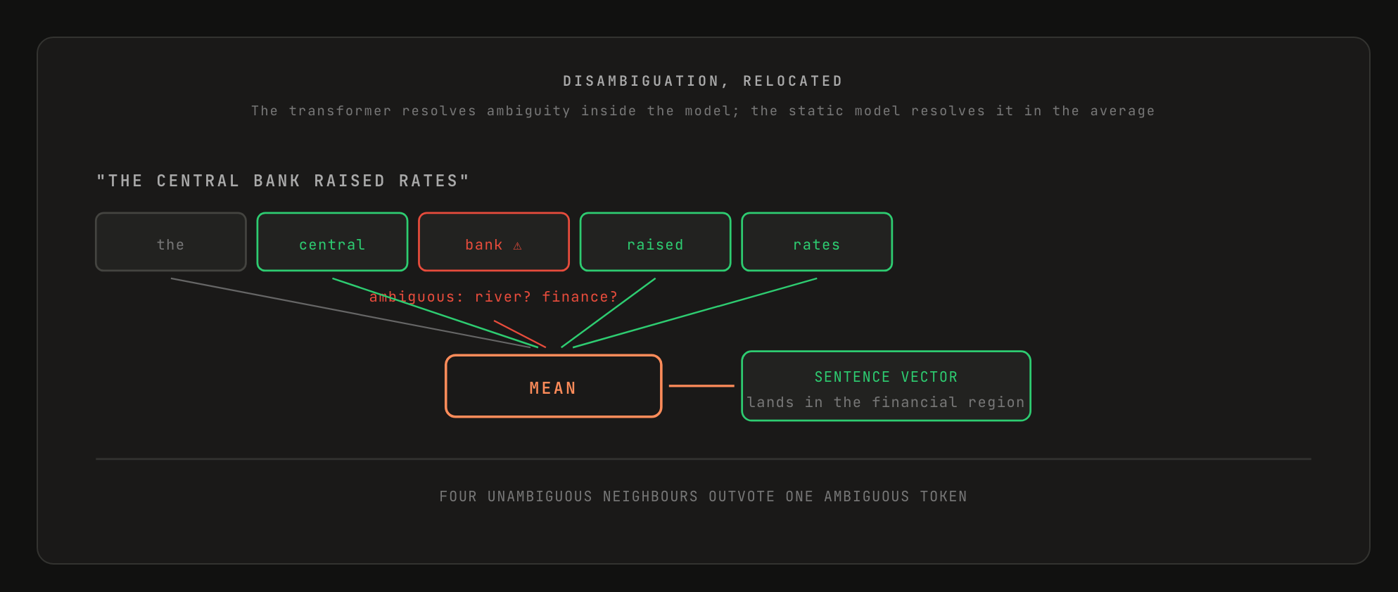
In a transformer, bank in “river bank” differs from bank in “central bank”; in a static model there is exactly one bank vector.
The load-bearing assumption is that the actual context provides enough disambiguation on its own. In “the central bank raised rates”, the ambiguous bank vector is averaged with central, raised and rates — themselves unambiguous — which pull the sentence vector firmly into financial territory.
Disambiguation still happens; it happens in the pooling rather than inside the network.
A precise footnote: the implementation multiplies each vector by its weight and then calls a plain mean — dividing by the number of tokens, not the sum of the weights. The two differ by a single scalar, so direction is identical and cosine similarity is unaffected; only magnitude changes, which matters solely for raw dot products or Euclidean distance on un-normalised vectors.
Takeaway. The mean is not a weakness bolted on; it is why the method is cheap. It fails predictably on very short inputs, on word order (a mean is order-invariant, so “dog bites man” and “man bites dog” are the same vector) and on negation.
09 The parts, decoded
| Component | What it is | Why it earns its place |
|---|---|---|
| Tokenizer | The teacher’s own subword tokenizer, carried over untouched | Defines the finite set that makes precomputation possible, and its frequency ordering is what Zipf needs. One artefact, two jobs. |
| Forward pass | Every vocabulary token pushed through the model; the output embedding is kept | Output beats input embeddings by ~6.1 points. The teacher must genuinely be a sentence transformer — plain BERT costs ~5.2 points. |
| PCA | Projection onto dominant axes of variation, 768 → 256 | +2.8 points and 3× smaller. Improves every task category, because it normalises the space as much as it compresses it. |
| Zipf weighting | Rank-derived weights via Zipf + SIF | +3.2 points for zero additional data or computation. Without it, function words swamp every sentence vector. |
10 Three ways to distill
| Mode | What it does | When to use it | Avg |
|---|---|---|---|
| Output | Encodes the model’s own subword vocabulary | The default. Quickest (~30s) and smallest (~30 MB). | 46.79 |
| Vocab (word) | Your own whole-word list | Drop-in replacement for GloVe / word2vec. No fallback for unseen words. | 48.58 |
| Vocab (subword) | Your words plus the subword vocabulary | Domain precision without losing coverage. Best measured. | 49.06 |
Vocabulary is free, speed-wise. Vocabulary-based models are larger in RAM, but all three modes run at identical speed, because cost is independent of vocabulary size. The decision is “do I have the RAM and do these terms matter”, never “can I afford the latency”.
11 Vocabulary as a lever
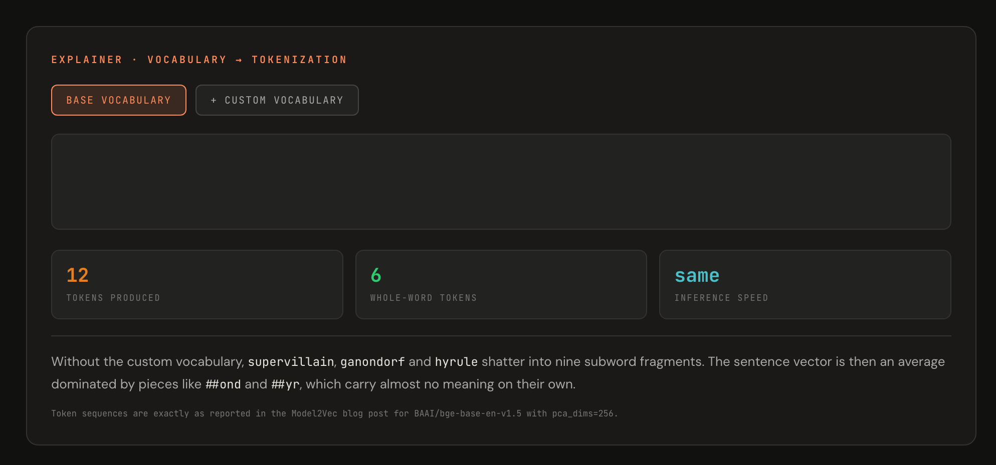
Take the sentence “supervillain Ganondorf has invaded Hyrule!”. Under the base tokenizer it becomes 12 tokens: supervillain → super + ##vill + ##ain, Ganondorf → gan + ##ond + ##orf, Hyrule → h + ##yr + ##ule.
Adding those three words to the vocabulary collapses it to 6 tokens.
Where the new vectors come from
The sentence transformer has never seen ganondorf, so where does its vector come from? Nothing is invented — the word is run through the teacher like every other entry. Since it is not in the tokenizer, it decomposes into subwords, and that whole sequence makes the forward pass:
# model2vec/tokenizer/tokenizer.py
token_id = vocabulary.get(token)
if token_id is not None:
    token_ids.append([*prefix, token_id, *suffix])   # already known -> a single token
else:
    token_ids.append(tokenizer.encode(token).ids)    # new word -> full subword decomposition
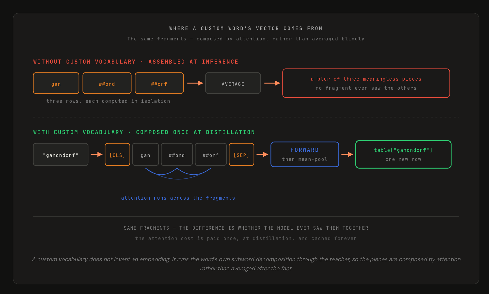
This is section 04’s idea, handed to the user. Feed the fragments through the model together and attention composes them into a representation of the whole word. Average three separately-stored fragment vectors and you get a blur of pieces that individually mean nothing.
Adding a word to the vocabulary caches that attention computation — paid once, kept forever.
12 The API surface
pip install model2vec
from model2vec import StaticModel

model = StaticModel.from_pretrained("minishlab/M2V_base_output")
embeddings = model.encode(["It's dangerous to go alone!", "It's a secret to everybody."])
from model2vec import distill

model = distill(model_name="BAAI/bge-base-en-v1.5", pca_dims=256)

# Add domain terms so they stop being shattered into subwords
model = distill(model_name="BAAI/bge-base-en-v1.5",
                vocabulary=["supervillain", "ganondorf", "hyrule"],
                pca_dims=256)
Model2Vec is supported directly in sentence-transformers via StaticEmbedding, so a static model slots into anything that already accepts a SentenceTransformer — LangChain, LlamaIndex, and anything built on them. It can also be trained there, keeping fast lookup-based inference.
13 Results on MTEB
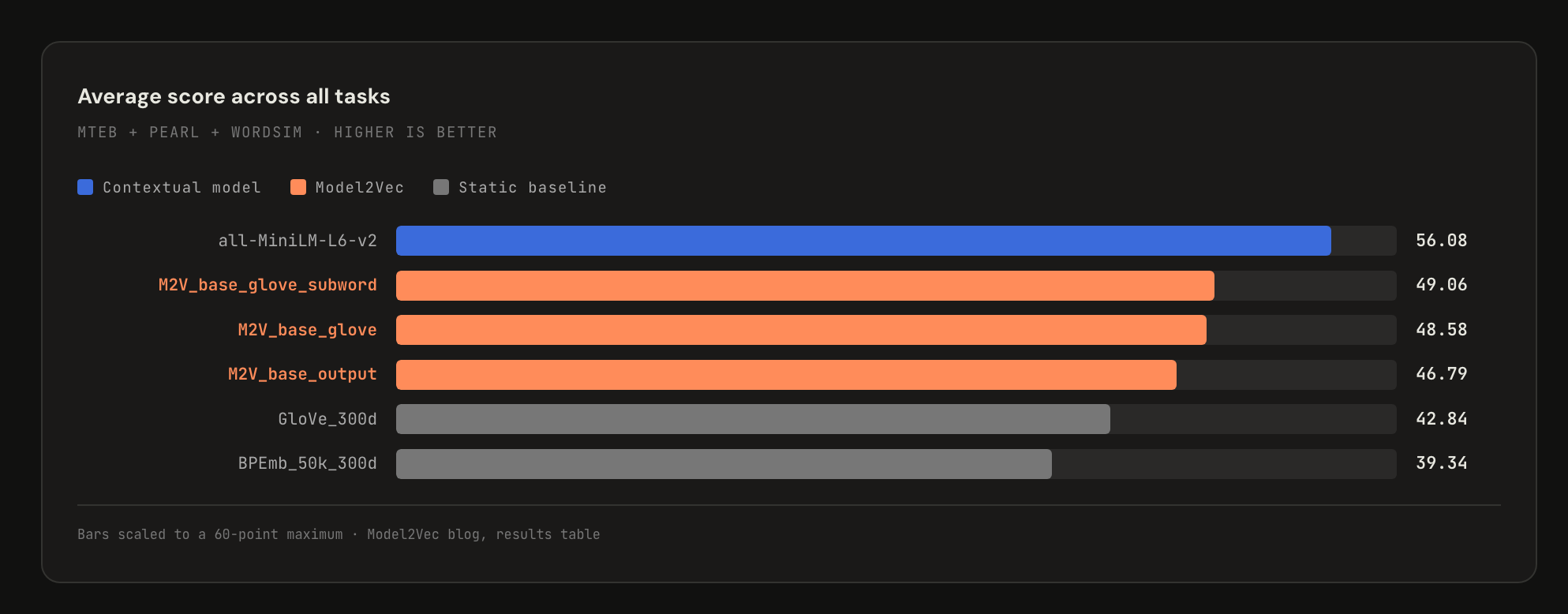
| Model | Avg (All) | Class | Clust | PairClass | Rank | Ret | STS | Pearl | WordSim |
|---|---|---|---|---|---|---|---|---|---|
| all-MiniLM-L6-v2 | 56.08 | 62.62 | 41.94 | 82.37 | 58.04 | 41.95 | 78.90 | 60.83 | 49.91 |
| M2V_base_glove_subword | 49.06 | 61.27 | 30.03 | 74.71 | 49.15 | 27.16 | 69.09 | 56.82 | 57.99 |
| M2V_base_glove | 48.58 | 61.35 | 30.52 | 75.34 | 48.50 | 29.26 | 70.31 | 50.28 | 54.29 |
| M2V_base_output | 46.79 | 61.25 | 25.58 | 74.90 | 47.63 | 26.14 | 68.58 | 54.02 | 49.18 |
| GloVe_300d | 42.84 | 57.31 | 27.66 | 72.48 | 43.30 | 22.78 | 61.90 | 45.65 | 43.05 |
| BPEmb_50k_300d | 39.34 | 55.76 | 23.35 | 57.86 | 43.21 | 17.50 | 55.10 | 47.56 | 41.28 |
Read across the columns and the shape of the trade becomes legible. On Classification the gap is small — 61.25 against 62.62. On Clustering (25.58 vs 41.94) and Retrieval (26.14 vs 41.95) it is severe.
That is exactly what the lack of context predicts: tasks needing a coarse regional signal survive; tasks needing fine distinctions do not.
The WordSim column is the one to notice — M2V_base_glove_subword scores 57.99 against MiniLM’s 49.91 and wins outright. For a single word there is no context to lose, and Model2Vec’s vectors come from a stronger teacher than GloVe’s co-occurrence statistics ever were.
14 Classification & the speed frontier
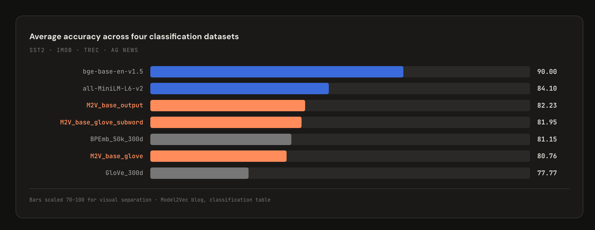
| Model | Average | SST2 | IMDB | TREC | AG News |
|---|---|---|---|---|---|
| bge-base-en-v1.5 | 90.00 | 91.54 | 91.88 | 85.16 | 91.45 |
| all-MiniLM-L6-v2 | 84.10 | 83.95 | 81.36 | 81.31 | 89.77 |
| M2V_base_output | 82.23 | 80.92 | 84.56 | 75.27 | 88.17 |
| M2V_base_glove_subword | 81.95 | 82.84 | 85.96 | 70.51 | 88.49 |
| BPEmb_50k_300d | 81.15 | 80.42 | 84.04 | 71.25 | 88.92 |
| GloVe_300d | 77.77 | 81.68 | 84.00 | 55.67 | 89.71 |
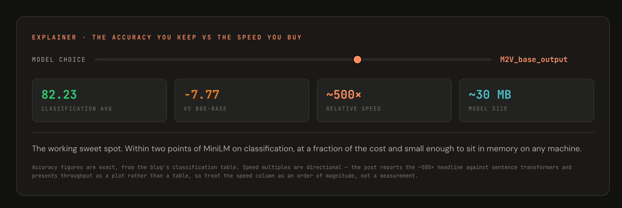
This is the strongest case for the method: M2V_base_output reaches 82.23 against MiniLM’s 84.10 — a gap of under two points — while being roughly 500× faster.
15 Ablations — what each trick buys
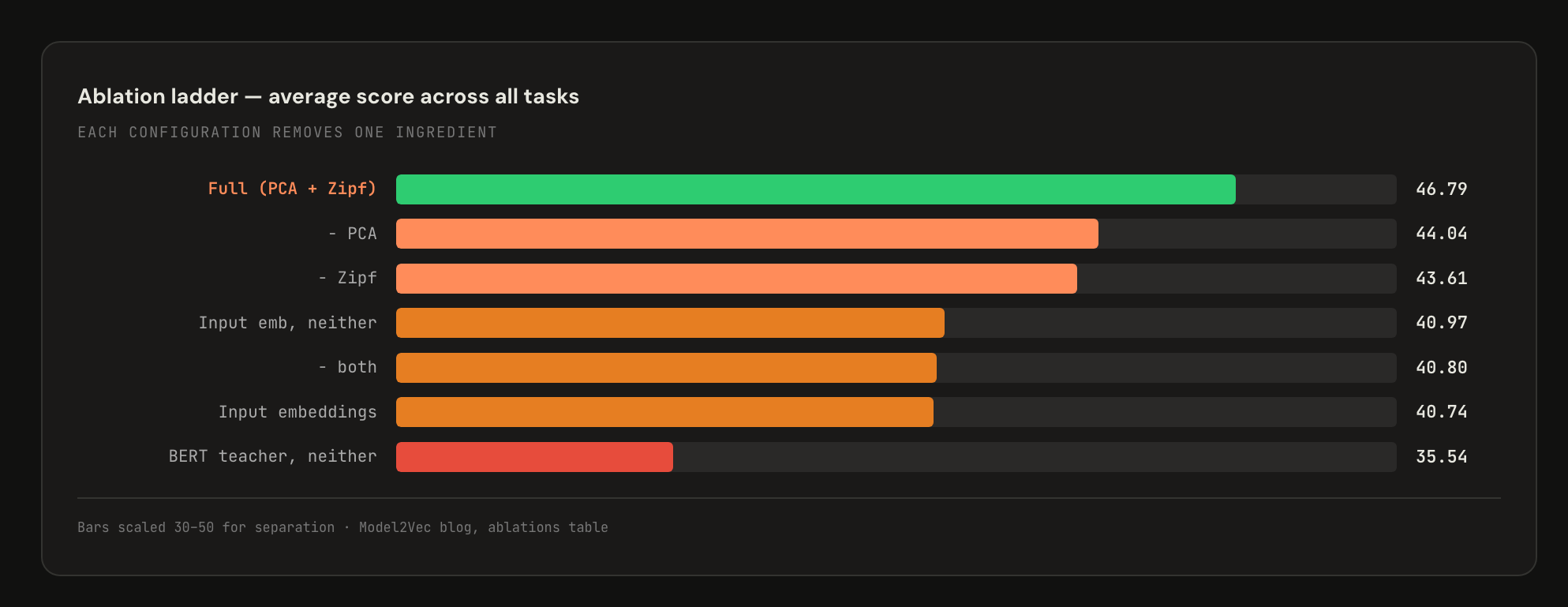
| Finding | Comparison | Worth |
|---|---|---|
| Output beats input embeddings | M2V_base_input (40.74) → M2V_base_output (46.79) | +6.1 |
| Teacher must be a sentence transformer | BERT (35.54) → BGE-base (40.80) | +5.2 |
| Zipf weighting | 40.80 → 44.04 | +3.2 |
| PCA | 40.80 → 43.61 | +2.8 |
BERT was trained on masked language modelling; its representations are excellent features but were never optimised so that cosine distance means semantic similarity. Sentence transformers are trained precisely for that, and since Model2Vec keeps nothing but the vectors and compares them geometrically, it inherits whatever geometry the teacher had.
Takeaway. The two largest effects are choices about what you extract; the two cheapest steps still carry six points between them.
16 When to reach for it
Reach for it when
- Volume dominates. Millions of documents, and embedding is the bottleneck.
- Latency is contractual. Single-digit-millisecond responses.
- You have no GPU. CPU-only serving, edge devices, cheap containers.
- You already use GloVe or word2vec. A strict upgrade on the same interface.
- Classification is the task. Under two points behind MiniLM.
- It is a first-stage filter. Narrow millions to hundreds, then re-rank properly.
Do not reach for it when
- Retrieval quality is the product. 26.14 vs 41.95 is not a rounding error.
- Clustering must be fine-grained. 25.58 vs 41.94.
- Word order carries meaning. A mean is order-invariant.
- Negation must be caught. “Safe” and “not safe” differ by one down-weighted token.
- Inputs are very short. No unambiguous majority to lean on.
- You only have a plain transformer. Costs ~5.2 points before you start.
The pattern underneath both lists. Does your task need to tell very similar texts apart, or only to place text in roughly the right region? Regional tasks survive the loss of context almost intact.
Discriminative tasks — retrieval, fine clustering, reranking — are exactly where context was doing the work.
17 Questions worth asking
Everything measured is zero-shot distillation. But Model2Vec models can be trained in Sentence Transformers, which raises the question of how much of the nine-point gap survives task-specific training.
The gap is concentrated in retrieval and clustering — exactly the tasks that benefit most from contrastive fine-tuning. The counter-argument is that training cannot restore what the architecture forbids: no amount of fine-tuning gives a static model two different vectors for the same token.
Nobody has published that decomposition.
The post attributes the +2.8 to normalisation rather than dimensionality reduction. If that is the full explanation, a cheaper normalisation step might capture the same benefit at full width, and compression becomes a separate decision about size.
If some of the gain genuinely comes from discarding low-variance noise, the two are entangled and there is an optimal dimensionality. No score-per-dimension curve is published. A supporting clue: the authors note input embeddings work better than expected and hypothesise it is because they are inherently normalised.
The assumption is fundamentally about having enough tokens to average, and must weaken as inputs shorten. Search queries are two or three words. Product titles are short. Chat messages are short.
These are also some of the most common places you would want a fast embedding model. A study of score against input length would show whether the sweet spot for static embeddings is genuinely the high-volume short-text case — or whether that is where the core assumption is weakest.
The BERT ablation proves the teacher matters — 5.2 points. The natural extrapolation is that better embedding models lift static models for free. But much of what makes a modern model better is better contextualisation, precisely what gets discarded.
If newer teachers improve mainly by handling context more cleverly, their per-token outputs may not be much better, and distilled students would plateau while teachers keep climbing.
Which holds determines whether static distillation rides the frontier or has a fixed ceiling.
18 The whole thing in one view
A transformer appears to handle unlimited text, but does so by decomposing it into a fixed vocabulary. A fixed set is enumerable, and an enumerable set can be precomputed exhaustively.
The apparently unbounded problem — embed any text — collapses into a bounded one. Every other property, including all the speed, descends from this.
Disambiguation does not disappear; it relocates. It moves from inside the network to the pooling step, where an ambiguous token is averaged with unambiguous neighbours. Attention did this precisely; the mean does it crudely; on ordinary sentences crude is enough.
On classification the gap to MiniLM is under two points.
A naive implementation scores 40.80; the real thing scores 46.79. The entire difference comes from two steps that take seconds and need no data. The lesson generalises: when you strip a learned system to its cheapest form, the geometry of what remains stops being self-correcting, and explicit normalisation and weighting must do the job the network was quietly doing.
Against MiniLM it loses by nine points, which sounds like a defeat. Against GloVe it wins by four and against BPEmb by seven, on every task, while being the same kind of object. Anyone considering Model2Vec has already decided they need static embeddings; given that, the only live question is which ones.
The single idea worth carrying away: the expensive part of an embedding model is recomputing things that never change, and the vocabulary is small enough to compute all of them exactly once.
19 Sources & methodology
Scores are exact — every number in the tables is copied from the post’s own results. Speed multiples are directional — the post gives a ~500× headline and presents throughput as a plot, so treat speed as an order of magnitude.
Size figures are exact arithmetic, computed from 32,000 tokens at 4 bytes per float32 value.
Several details here were verified against the model2vec source rather than the post: the per-entry encoding and mean pooling, the Zipf/SIF weight formula and its real-vocabulary behaviour, why weights are stored separately from vectors, and how custom-vocabulary words receive their vectors.
- Hugging Face blog: Model2Vec
- model2vec on GitHub
- MinishLab on Hugging Face
- MTEB leaderboard
- Sentence Transformers
Attribution. Model2Vec is the work of Thomas van Dongen and Stéphan Tulkens (MinishLab), with the Sentence Transformers integration contributed by Tom Aarsen. This page is an independent explanatory rendering of their published post; all credit for the method and the results belongs to them.